Fast Robots: Lab 12

In lab 11, we have built a localization algorithm with Bayes filtering method. We were working with a virtual robot in a simulation environment. In each unit of robot movement, the localization algorithm incorporates both the odometer readings and the sensor readings when making a 360 degree turn in place to make an estimate of the robot's state. As I have demonstrated in lab 11, this localization method works surprisingly well.

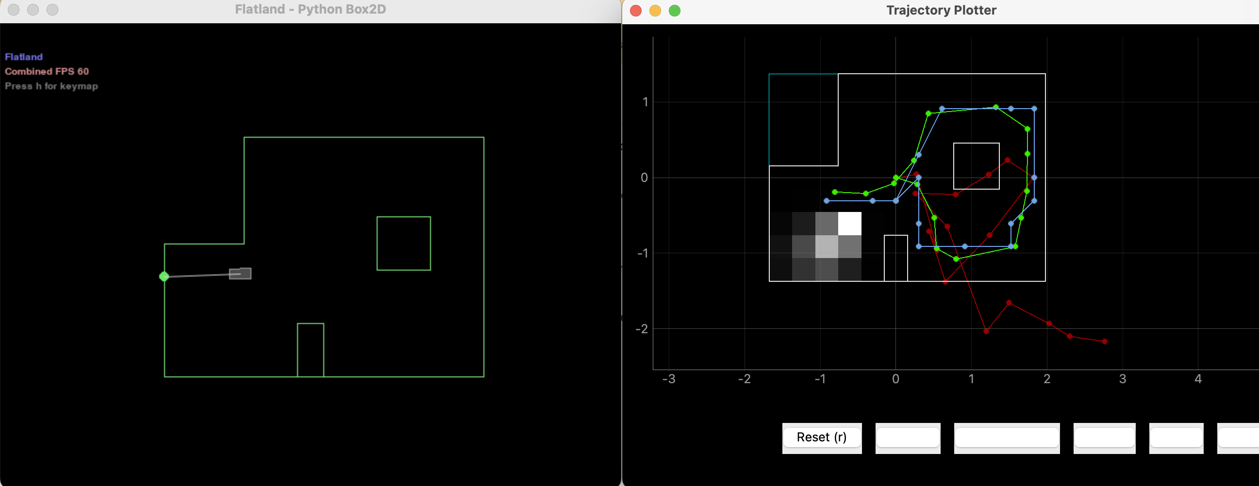
However, everything happened in lab 11 is inside simulation environment. In this lab, we will incorporate the real robot in a real map, and try to do localization with it. The localization task performed in this lab is simplified. The robot will be manually placed in one of the four spots in the map, and it will turn in place 360 degrees when it receives a command from the laptop. When it is turning in place, it will take a ToF measurement every 20 degrees (that is 18 measurements in total). The robot will then transmit the ToF sensor readings back to the laptop. The laptop will run the Bayes algorithm to perform localization of the robot. Because the robot is not moving, it will start with a uniform prior belief, and it will run the update step of the Bayes filter algorithm to estimate the location of the robot.

Implementation

Because the robot and my laptop need to work together in this lab, I am dividing the implementation into two parts: robot implementation and Python implementation.

Robot (embedded Arduino) implementation

Three BLE robot commands are added for this lab:

MAKE_OBSERVATION: the robot will turn in place for 360 degrees (counter-clockwise) in 20 degree steps. The robot takes a ToF measurement every 20 degree, and stores the ToF measurements in a local array. A total of 18 measurements are taken.
RESET_OBSERVATION: resets all the global variables used in MAKE_OBSERVATION. This command needs to be called between two MAKE_OBSERVATION procedures. Otherwise a hardware reset is required.
READ_ARR(ARR_IDX, ELEMENT_IDX): the way to read data on the robot. The first argument, ARR_IDX, specifies which array to read. In this context, there is only one array, so this argument will be 0 when called. The second argument, ELEMENT_IDX, specifies which element to read in the corresponding array. The robot will update the TX_FLOAT characteristic after this command is called, and the value can be read by laptop. The laptop reads the entire array by iterating ELEMENT_IDX.

Implementation of MAKE_OBSERVATION is straight-forward. Code reusing from lab 9: Mapping is the key. PID control is used to control the orientation of the robot. Gyroscope-accumulated yaw is used as PID input. When a measurement is taken, the robot stores the values in an array that is living in program stack.

RESET_OBSERVATION simply resets all the flags, indexing variables, and temporary arrays. If RESET_OBSERVATION is not called between two calls of MAKE_OBSERVATION, the second call of MAKE_OBSERVATION will not work (or it will, but with undefined behavior).

I found that using READ_ARR(ARR_IDX, ELEMENT_IDX) to retrieve array values is better than using event handler in Python. Using the event handler (with BLE notification) in Python is tricky: we will need to use the async feature inside Jupyter Notebook. I am no expert of either async or Jupyter Notebook, so even though switching to READ_ARR means rewriting of all my previous BLE code, I am doing to reduce the risk of hitting issues that will take much longer time to resolve.

Here is a code snippet of how the READ_ARR function works in the Artemis board.

                            
case READ_ARR:
Serial.println("Command READ_ARR triggered");
int read_arr_type, read_idx;

// Extract the next value from the command string as an integer
success = robot_cmd.get_next_value(read_arr_type);
if (!success)
    return;

// Extract the next value from the command string as an integer
success = robot_cmd.get_next_value(read_idx);
if (!success)
    return;

// send back the array index to be read
if (read_arr_type == 0){
    tx_characteristic_float.writeValue(ble_tof_data[read_idx]);
}
else if (read_arr_type == 1){
    tx_characteristic_float.writeValue(ble_angle_data[read_idx]);
}

break;

Python implementation

Python implementation is also straight-forward. The instructors have provided a framework in a class RealRobot. This class has a function perform_observation_loop, and it is all that we need to implement. This function takes no arguments, and it returns a column numpy array of the range values in meters. Assuming that the robot's microcontroller has all the commands implemented correctly, this Python function will only need to do the following things:

Use RESET_OBSERVATION command to prepare the subsequent call of MAKE_OBSERVATION.
Use MAKE_OBSERVATION command to tell the robot to begin spinning in place and taking observations.
Sleep for some time to let the robot finish its measurements
Use READ_ARR command to get all the measurement values

Here is a code snippet for the implementation of perform_observation_loop.

                            
def perform_observation_loop(self):

    # Connect to the Artemis Device
    ble.connect()

    # reset observation
    ble.send_command(CMD.RESET_OBSERVATION, "")

    # trigger data collection
    ble.send_command(CMD.MAKE_OBSERVATION, "")

    # sleep for collection to complete
    time.sleep(25)

    # get array length
    ble.send_command(CMD.GET_ARR_LENGTH, "")
    num_samples = ble.receive_float(ble.uuid['RX_FLOAT'])

    # iterate over tof data and angle data. get both
    tof_data = []
    angle_data = []

    for i in range(int(num_samples)):
        ble.send_command(CMD.READ_ARR, f"0|{i}")
        tof_data.append(ble.receive_float(ble.uuid['RX_FLOAT']))

        ble.send_command(CMD.READ_ARR, f"1|{i}")
        angle_data.append(ble.receive_float(ble.uuid['RX_FLOAT']))

    # Disconnect
    ble.disconnect()

    # sanity check print tof sensor readings
    print(tof_data)

    return np.array(tof_data)[np.newaxis].T / 1000, np.zeros((1,1))

Note that my code has one more command implemented: GET_ARR_LENGTH. This is optional. This command gets the length of the array from the microcontroller. It simply makes the code easier to maintain.

The video below shows the process of doing one localization. Python on my laptop starts running first, then the robot receives the MAKE_OBSERVATION command and starts spinning and taking measurements. After that is finished, Python reads the array, passes it into the already-exists localization code, and displays both the estimated location (blue dot) and the ground truth location (green dot) on the plotter.

Video of the robot doing localization in spot (5, 3, 0). The Python running on my laptop triggers the robot to make an observation loop. ToF sensor measurements are transmitted to the laptop afterwards, and the laptop runs the Bayes filter update step to make a prediction of the robot's state. Both the ground truth (green dot) and the estimate position (blue dot) are plotted in the virtual map.

Localization in 4 spots

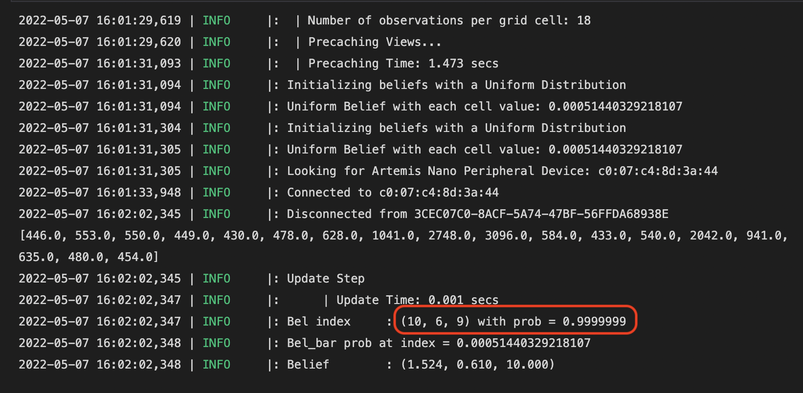
Next I am going to present the results when doing localization in the four required spots: (-3, -2, 0), (0, 3, 0), (5, -3, 0), (5, 3, 0). For each spot, I am presenting the plotter map view and the LOG messages. I will also discuss how close the estimate is from the ground truth and the results.

Spot #1 (-3, -2, 0)

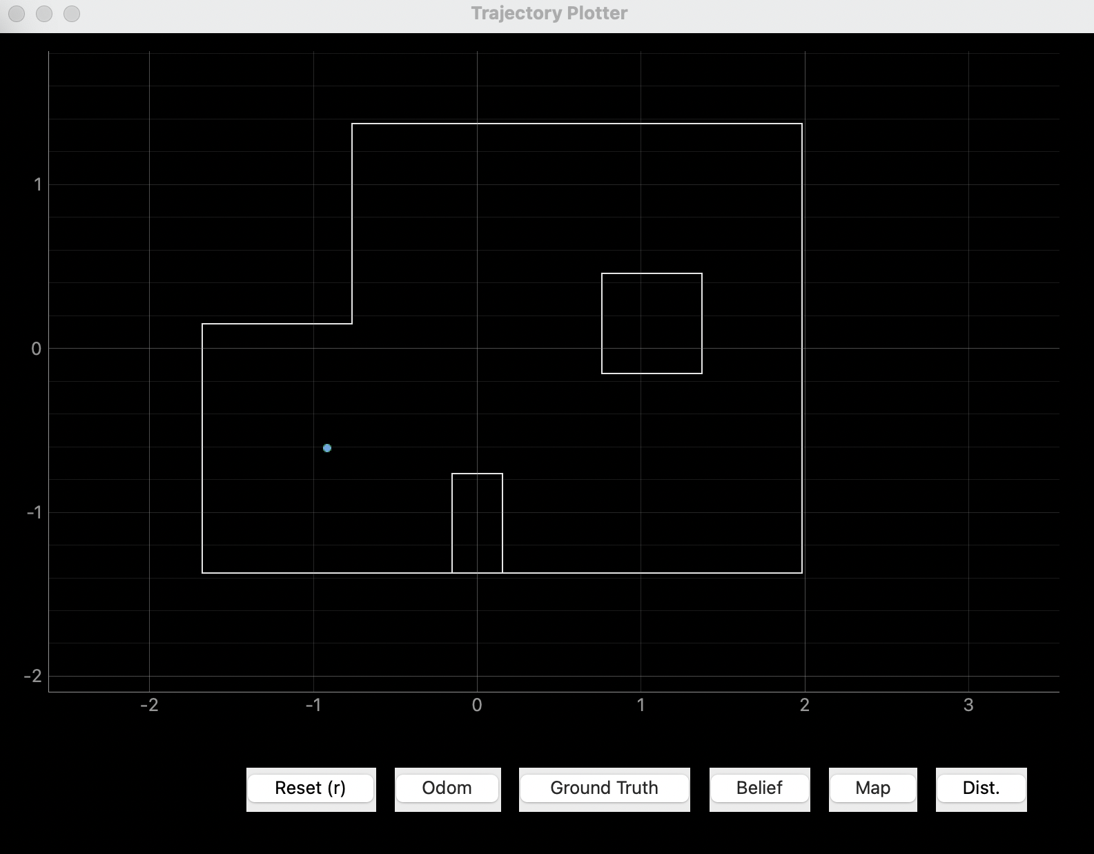
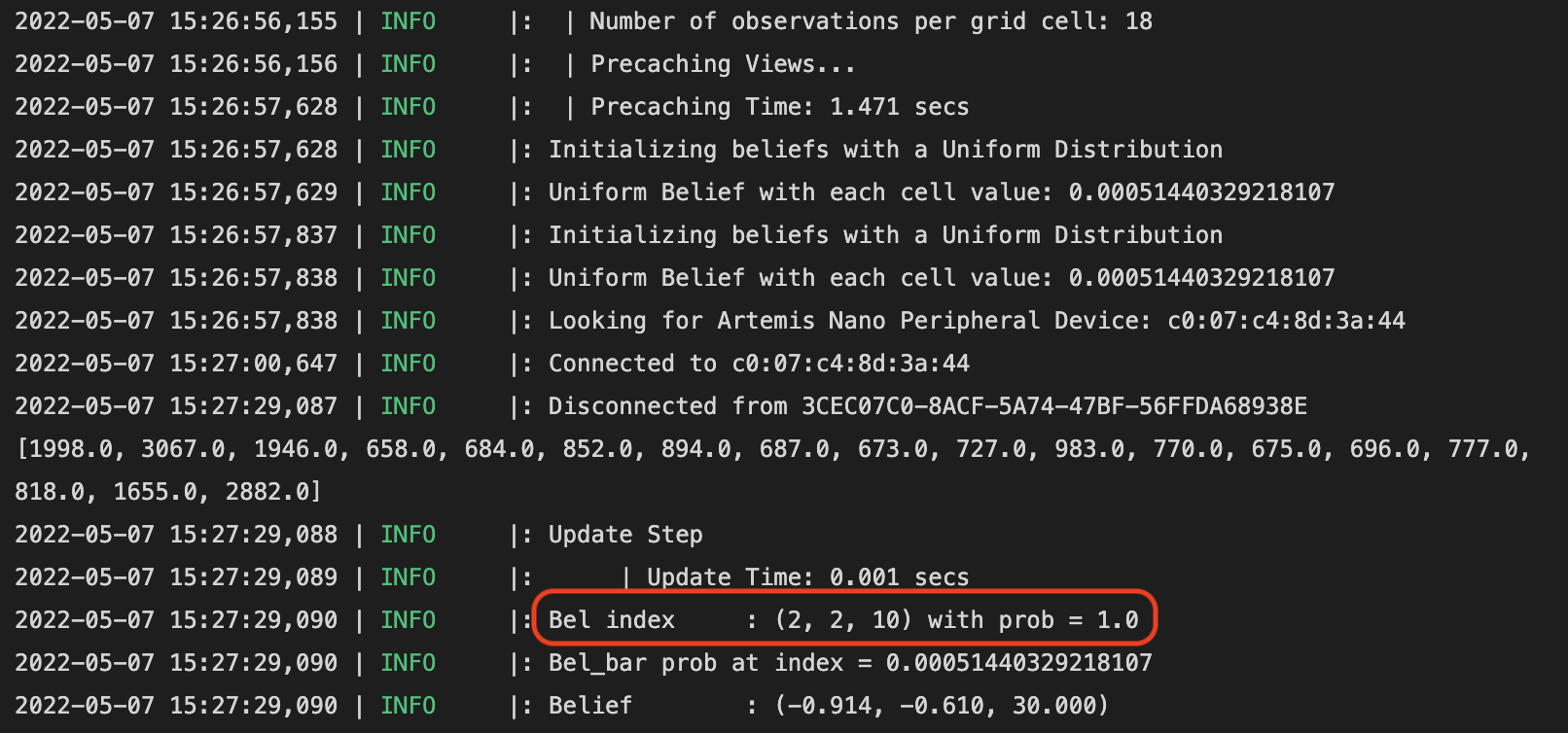
For this spot, we only see the blue dot (estimated state) on the plotter. This is because the estimated state is the same as the ground truth state. However, since the plotter map only shows the x, y location, we also need to check the LOG message to make sure the orientation is correct as well. From the LOG message, we see that the yaw index is 10, which corresponds to degree 20. The correct orientation should be 0 degrees. There is this 20 degree difference between the ground truth and the localization estimate. I would argue that this is very good results, considering the gyroscope-accumulated yaw could drift when taking measurements, and the ToF sensor is, after all, not that accurate. Another reason being that an offset of 20 degrees in orientation would only result in 1-cos(20 degrees) = 6% difference of the ToF measurement, which is close to the error band of the ToF sensor.

Spot #2 (0, 3, 0)

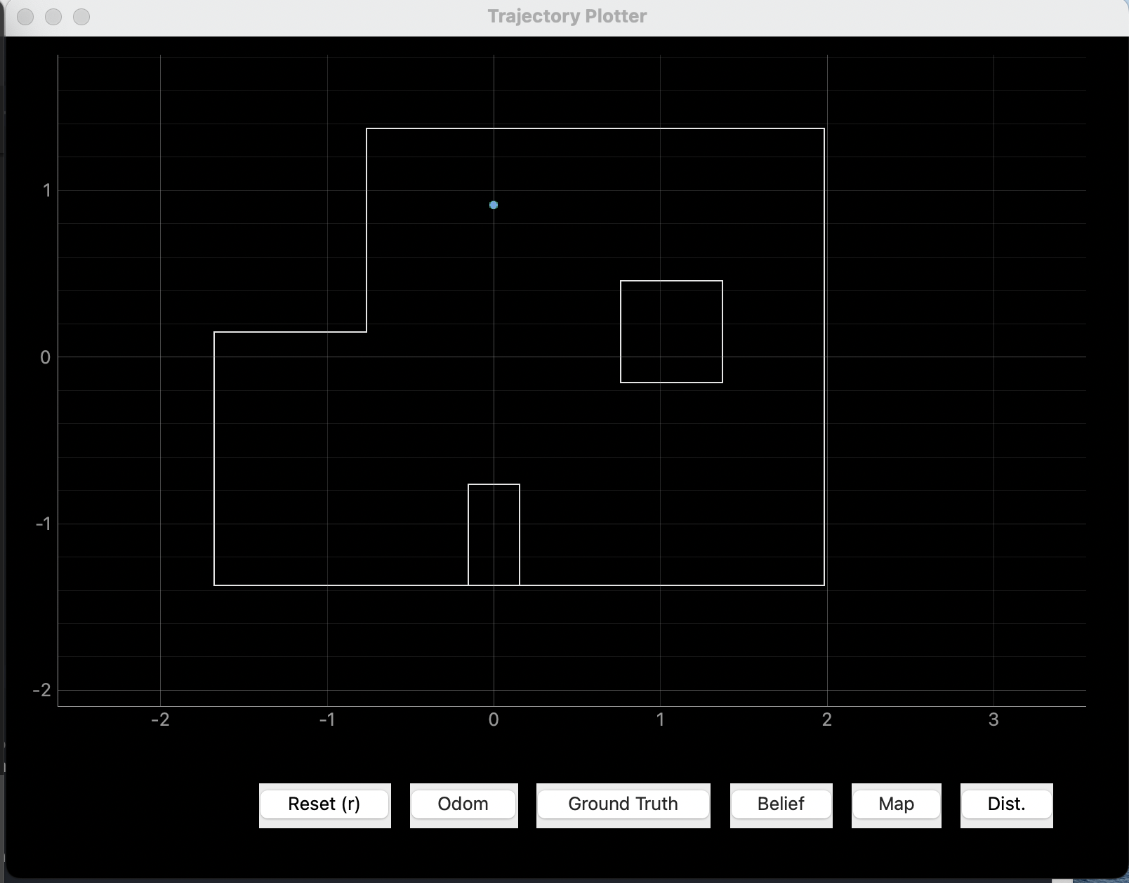
The results from this spot is similar to that in the last spot. We see on the plotter that the ground truth and the Bayes estimate overlaps, meaning that x, y estimates is identical. However, the yaw index is 8, which corresponds to -20 degrees. I call this very good result as there are errors in the ToF sensor and gyroscope. Same reason as in the last spot.

Spot #3 (5, -3, 0)

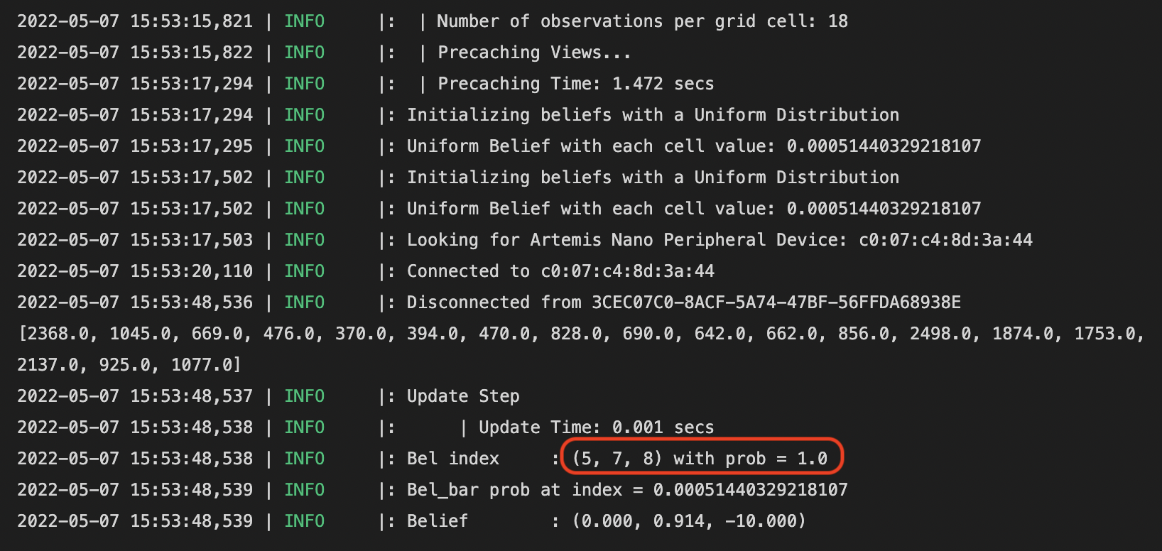
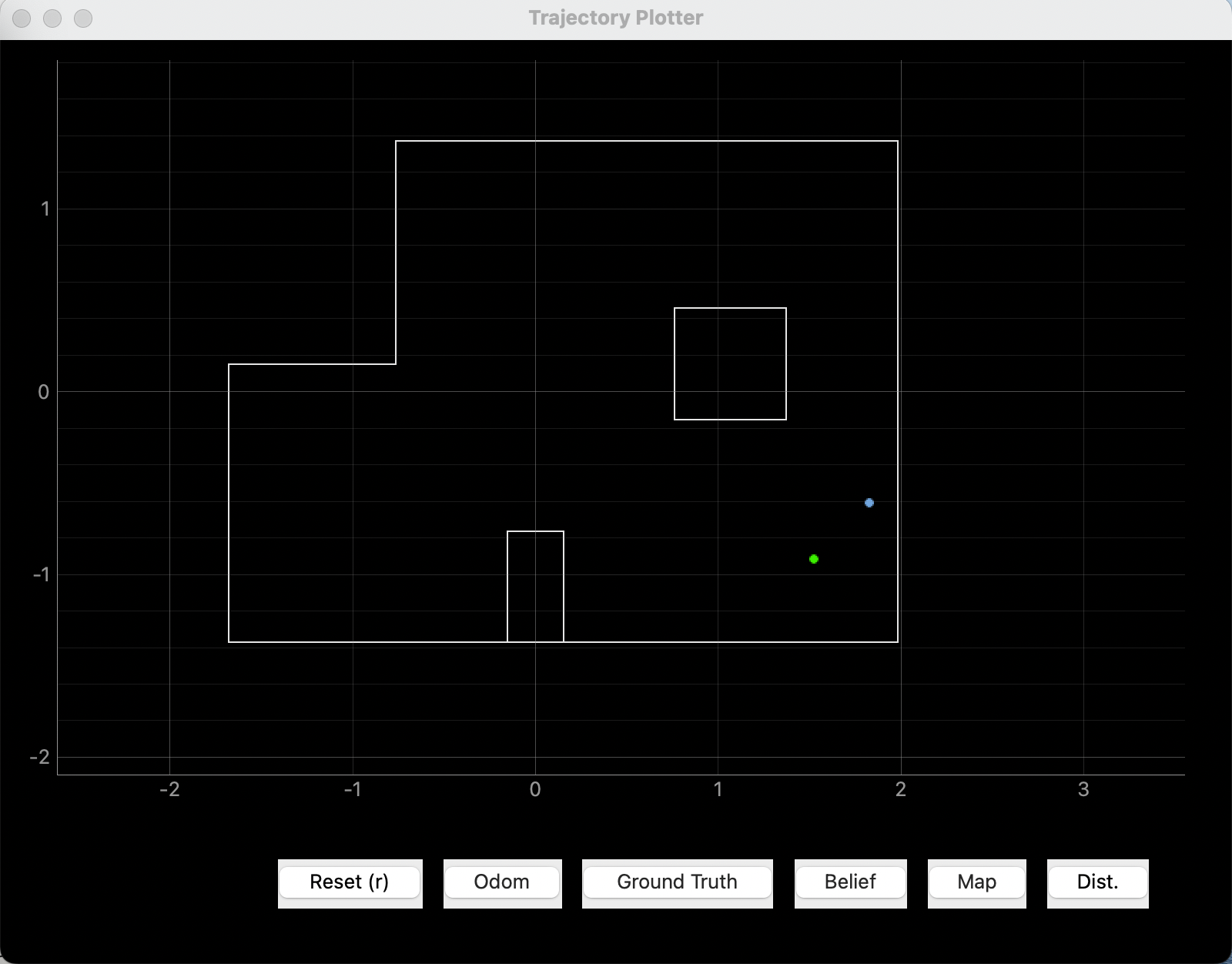
This time we can see that the x, y, yaw states are all different between the Bayes estimate and the ground truth. However, we can see from the LOG message that the yaw angle is not that far off. In addition, the x, y 2d location is also very close to the ground truth. In addition to sensor errors, the reason of this slightly off estimate could be that the robot is far from the walls in the north direction and the west direction. When the wall is far away, ToF sensor readings become less reliable and less accurate. I believe this error is reasonable given the capabilities of the ToF sensor.

Spot #4 (5, 3, 0)

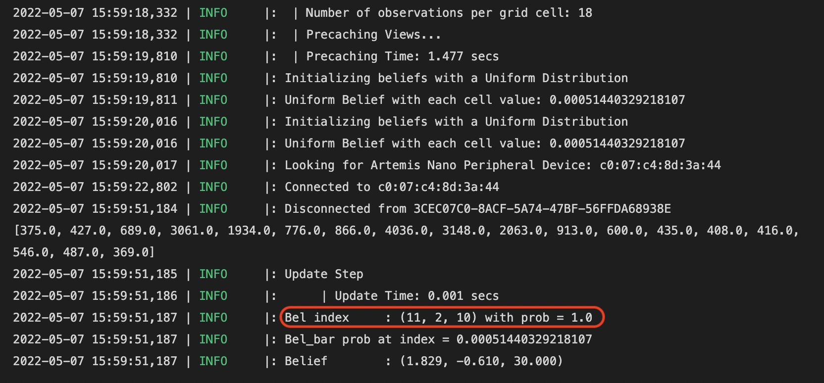
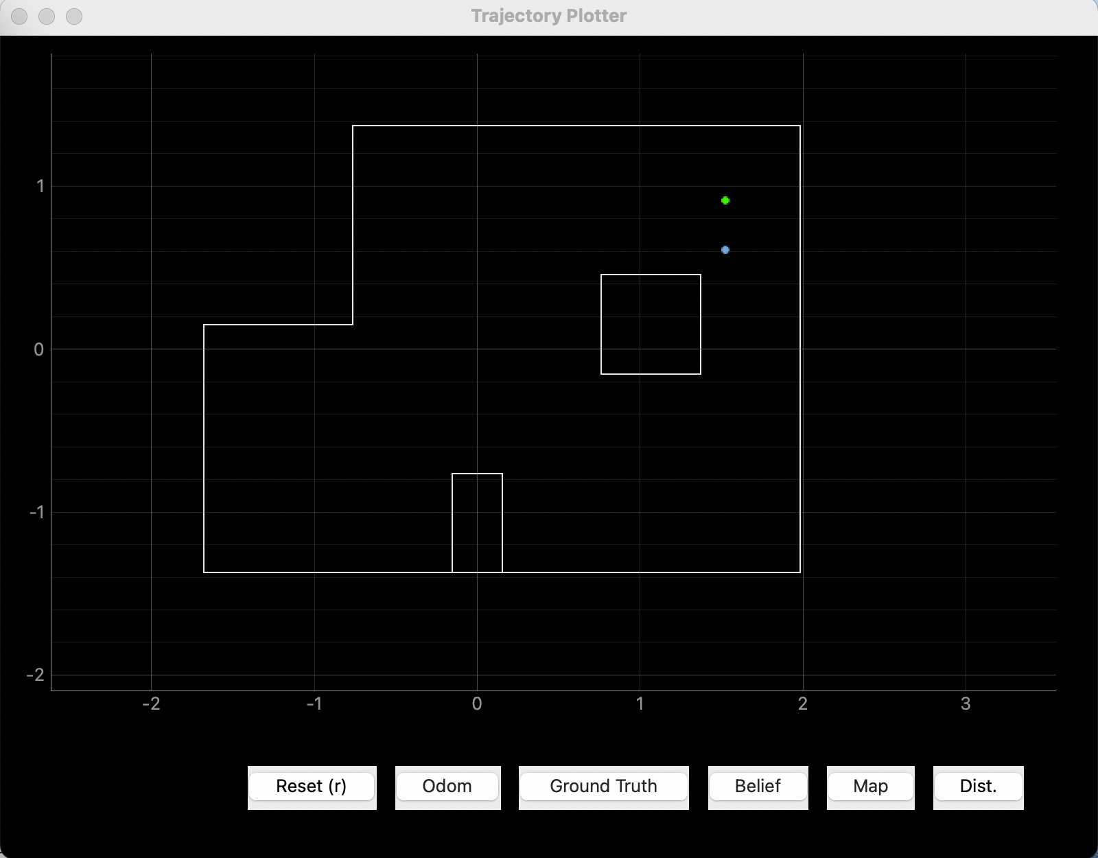
In this estimate, the yaw angle is correct (index = 9 same as angle = 0 degrees). The x position is also correct, but the y position is off by one grid. I believe this is very reasonable as the south wall is very, very far away from the robot, and it is reaching the limit of the ToF sensor's ranging length. Even though the north and east walls are close to the robot, the error measurements in the south direction could dominate.

In summary, is this lab successful? I think so because the Bayes estimates are not far away from the robot's ground truth, and both the ToF sensor and the gyroscope are not the most accurate ones. This leads to another question: do I trust this localization model enough such that I will use it for lab 13? Probably not since the "turning in place" action will actually change the yaw angle of the robot. and if the robot is to travel a long distance in each step, then any errors could be catastrophic for the robot's route.

Localization (real)

From simulation to reality