The purpose of this lab is to implement robot localization using Bayes filter. This lab is built on previous labs, including the mapping lab where we used the robot to measure outside environment and recreate a line-map, and the simulator lab where we have get familiar with using the simulator. In this lab, we are working only with the simulator, which contains the same map as the real-world map. We will implement our Bayes filter algorithm on the virtual robot in the simulator.
The rationale behind starting with the simulator instead of going straight into using the physical robot is that debugging with the simulator is much easier. We would like to make sure the Bayes filter algorithm software is implemented correctly. Then in the next stage (the following lab), we can focus on getting the communication between the robot and the laptop correct. This way, we will not have to deal with a possible difficult situation where we are debugging the robot and the algorithm at the same time...
Localization goal and state space
Localization and the map
In robotics, localization simply means determining the state (which in the context of this lab, the location and orientation) of the robot without involving a human. Otherwise, I can certainly look at (or measure) the true state of the robot and send such information to the robot. In this lab, the robot travels inside a 2D map (refer to lab 9: mapping). It could be in any (x, y) location inside the map, and it could be facing any direction. To quantify the state in mathematical notation, the robot's state can be described in (x, y, theta), where
- [-1.6764, +1.9812) meters or [-5.5, 6.5) feet in the x direction,
- [-1.3716, +1.3716) meters or [-4.5, +4.5) feet in the y direction,
- [-180, +180) degrees along the theta axis.
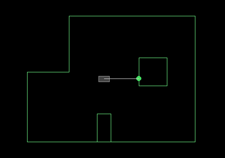 The virtual robot inside the simulator. The robot's state is (0, 0, 0).
If the robot turns slightly to its left, it's
 theta increases. If the robot turns slightly to its right, then it's theta decreases.
Discretized 3D grid space
Due to the nature of modern electronics being mostly digital, it is very difficult to deal with the continuous, analog state space. Therefore, we will discretize the robot's state space to make it computationally feasible. We will make the continuous 3D space into 3D grid space, with each grid being in size (0.3048m, 0.3048m, 20 degrees) The size of the grid cell in (x, y) coordinates is the same as the tile grid cell's size. The total number of cells along each axis are (12, 9, 18). Simple calculations will tell us that the robot in the previous picture is sitting in grid cell index (5, 4, 8).
In our Bayes filter implementation, we will maintain a 3D array of dimensions (12, 9, 18). We call this the belief array. The value of the array cell with index (x, y, a) represents the probability of the robot being in discretized state (x, y, a). The picture below shows a visualization of the 3D grid cell array.
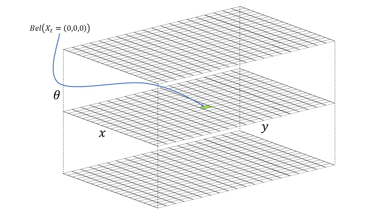 3D visualization of the discretized state space.
During the course of robot movements and Bayes filter updates, the Bayes filter algorithm will update the probability of the robot's presence in each grid cell. The grid cell with the highest value (thus highest probability) represents the most probable pose of the robot.
Bayes filter algorithm
In our experiment, the robot progress in steps. In each step, the robot does the following two things:
- Make a movement characterized by the odometry motion model. A movement can be described by three parameters:
rotation1, translation, rotation2. - Make an observation by turning 360 degrees in place and taking a ToF sensor measurement every 20 degrees, yielding an array of 18 distance measurements.
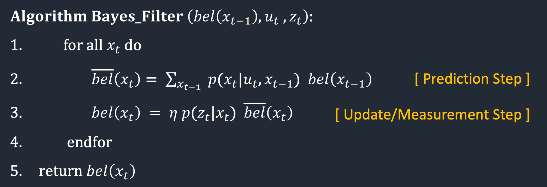 Bayes filter algorithm
x_t describes the state of the robot in timestep t. There is a unique x_t corresponding to a set of index in the 3D grid space. bel_bar(x_t) means the prior belief of the possibility of a robot being in state x_t, and bel(x_t) means the belief of the possibility of a robot being in state x_t. The algorithm has two steps, the prediction step, and the update/measurement step.
In the prediction step (line 2), the Bayes filter algorithm computes the prior belief for the current timestep (that is bel_bar(x_t)) from the belief in the previous timestep (bel(x_t)) and the control input of the robot (u). Because the control input of the robot will not be available until robot action 1 is completed, the prediction step will be executed, in each timestep, after robot action 1 is executed. The calculation in the prediction step is simple conditional probability. In words, for each x_t, the algorithm sums up the probability of transitioning from all the previous possible states (in bel) given the last robot control action.
In the update step (line 3), the Bayes filter algorithm incorporates the ToF observation measurements into its estimation. Note that in the prediction step, only information from the robot's control input is taken into account. What happens in the update step is that for each x_t, the robot multiply the prior belif in bel_bar with the likelihood of the robot making the measurements in the state. bel is then normalized such that probability sums to 1.
Code walkthrough
In this section, we will look at my implementation and the Bayes filter algorithm together, such that we can relate the implementation with the algorithm.
The first thing to mention is a helper function yaw_to_deg(yaw_idx). It takes the angle grid index as input, and returns the angle (in degrees) corresponding to this angle index.
 yaw_to_deg helper function
Moving on, there is this compute_control(cur_pose, prev_pose) function. It takes two arguments, two states in the form of (x, y, yaw), and calculates the odometry control needed for moving the robot from prev_pose to cur_pose. The returned odometry control is in the form of (rotation_1, translation, rotation_2). rotation_1 and rotation_2 are normalized to be in the range of [-180, 180] in line 42 and 43.
This function is needed because recall in line 2 of the Bayes filter algorithm, the control input is needed instead of two positions.
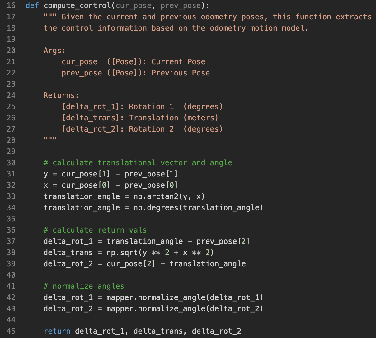 compute_control function
To calculate p(x_t | u_t, x_t-1) in the update step of the Bayes filter algorithm, we use this odom_motion_model(cur_pose, prev_pose, u) function. The argument u is the actual control input. The arguments cur_pose, prev_pose are two states of the robot. This function calculates the probability of transitioning from prev_pose to cur_pose given the actual input, u. The probability is calculated using gaussian distribution with the mean being the actual input and the deviation being odom_rot_sigma [default=15] and odom_trans_sigma [default=0.45], evaluated at the calculated control needed by transitioning from prev_pose to cur_pose (line 62-64).
 Equations to calculate the probability of transition from one state to another given a control
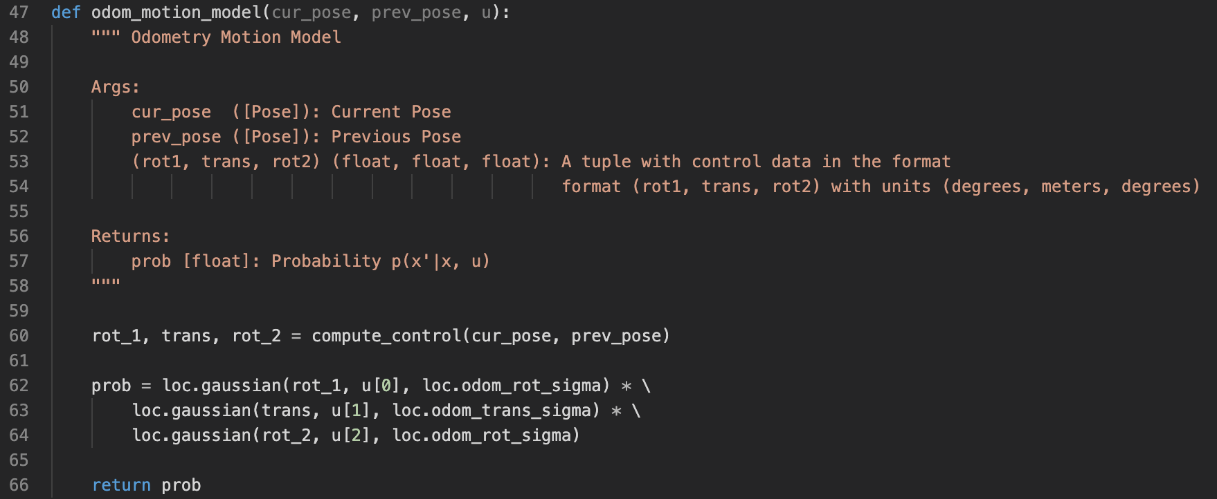 Implementation of the odometry motion model
With compute_control and odom_motion_model being implemented, we can implement prediction_step(cur_odom, prev_odom). The actual input, u, is first calculated by calling compute_control. Then bel_bar is reset to zeros. Then the algorithm steps over all the possible state pairs to update values in bel_bar following the Bayes prediction step algorithm. p(x_t|u_t, x_t-1) is calculated by calling the odom_motion_model function, and bel is an array available for access.
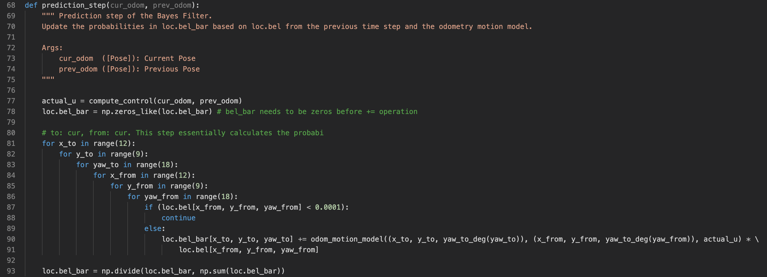 Implementation of Bayes algorithm's prediction step
In the update step, we have the equation of bel(x_t) = p(z_t|x_t) * bel_bar(x_t) from the Bayes filter algorithm. p(z_t|x_t) signifies the probability of the robot getting measurement z_t if it is in the state x_t. This value is calculated by calling the sensor_model function, which we will discuss later. The other neede value, bel_bar(x_t), is available after running the prediction step, and it will simply be an array available. At the end, bel is normalized to have the probabilities sum to 1.
 Implementation of Bayes algorithm's update step
Last but not least, we need to discuss the sensor model. sensor_model(obs, pos) takes two arguments. obs is an 1D array of length 18, corresponding to the 18 measurements the robot took in observation step. The second argument pos is an index in the 3D grid space. This function returns an 1D array of length 18, each element represents the likelihood of getting this sensor reading given the robot is in state pos. The returned array is multiplied together in update_step to get p(z_t|x_t).
 Algorithm of the sensor model
Again, the sensor model uses gaussian to calculate the probability. For each sensor measurement, the function first fetches the true measurement (calculated offline by ray-tracing), then it evaluates with a gaussian, with mean as the true value, and deviation as sensor_sigma [default=0.1], evaluated at the observed value (line 113).
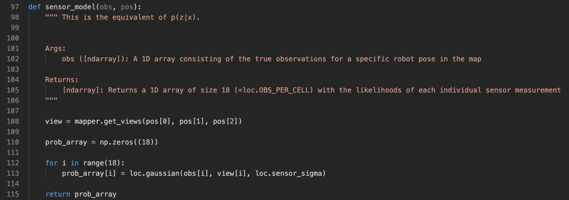 Implementation of the sensor model
Result and outcomes
Below are two videos showing the results when running my Bayes filter algorithm on the simulator. The robot travels following a trajectory. There are three trajectories on the plotter. The red one is the odometry reading, which is very not accurate. The green one is the ground truth position of the robot, and the blue one is the location of the robot from running Bayes filter algorithm. In the second video, the plotter has the marginal distribution of prior belief overlayed on the screen.
Both videos shows very promising results. The odometry readings are way off the ground truth, but the Bayes filter prediction (the blue line) follows the ground truth (the green line) very closely. This has convinced me the correctness of my implementation. If my implementation is still not correct, this will still be good enough :)
Robot localization #1 Robot localization #2 (with marginal distribution in the 2d grid space)